Fitting wells#
This notebook introduces the concept of fitting wells and how they are used in gwrefpy. The methodology originates from the description by its author Strandanger (2024).
This notebook can be downloaded from the source code here.
To analyse deviations in groundwater level timeseries, the gwrefpy methodology relies on observation wells and reference wells. To check for deviations in an observation well, we fit its data to a reference well using regression. When fitting the two wells, we specify a calibration period. If data outside of the calibration period does not follow the fitted regression, a deviation has occurred.
In this notebook, we will dive deeper into the fitting workflow and showcase this library’s associated capabilities.
Note
import gwrefpy as gr
import pandas as pd
import matplotlib.pyplot as plt
import warnings
warnings.filterwarnings("ignore")
gr.set_log_level("ERROR")
plt.set_loglevel("ERROR")
Data#
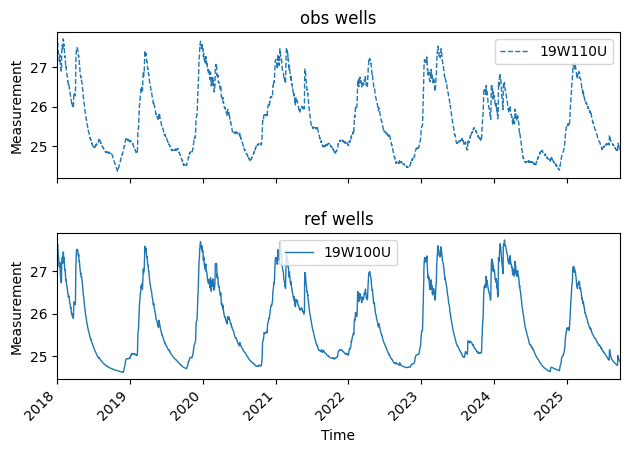
In this notebook, we will work with data provided by gwrefpy. Let’s load the model using its file name and plot the observation well and reference well separately.
model = gr.Model("deviation_example.gwref")
model
Model(name='deviation example', wells=2, fits=0)
Anatomy of a fit#
Let’s walk through the anatomy of a fit by fitting the observation well 12GIPGW to the reference well 45LOGW. To fit wells within a model, we call model.fit() which has the following signature:
help(model.fit)
Help on method fit in module gwrefpy.fitbase:

fit(obs_well: gwrefpy.well.Well | list[gwrefpy.well.Well] | str | list[str], ref_well: gwrefpy.well.Well | list[gwrefpy.well.Well] | str | list[str], offset: pandas._libs.tslibs.offsets.DateOffset | pandas._libs.tslibs.timedeltas.Timedelta | str, aggregation: Literal['mean', 'median', 'min', 'max'] = 'mean', p: float = 0.95, method: Literal['linearregression'] = 'linearregression', tmin: pandas._libs.tslibs.timestamps.Timestamp | str | None = None, tmax: pandas._libs.tslibs.timestamps.Timestamp | str | None = None, report: bool = True) -> gwrefpy.fitresults.FitResultData | list[gwrefpy.fitresults.FitResultData] method of gwrefpy.model.Model instance
    Fit reference well(s) to observation well(s) using regression.

    Parameters
    ----------
    obs_well : Well | list[Well] | str | list[str]
        The observation well(s) to use for fitting. Can be Well objects,
        well names (strings), or lists of either. If a list is provided,
        each well will be paired with the corresponding reference well by index.
    ref_well : Well | list[Well] | str | list[str]
        The reference well(s) to use for fitting. Can be Well objects,
        well names (strings), or lists of either. If a list is provided,
        each well will be paired with the corresponding observation well by index.
    offset: pd.DateOffset | pd.Timedelta | str
        The offset to apply to the time series when grouping within time
        equivalents.
    aggregation: Literal["mean", "median", "min", "max"], optional
        The aggregation method to use when grouping data points within time
        equivalents (default is "mean").
    p : float, optional
        The confidence level for the fit (default is 0.95).
    method : Literal["linearregression"]
        Method with which to perform regression. Currently only supports
        linear regression.
    tmin: pd.Timestamp | str | None = None
        Minimum time for calibration period.
    tmax: pd.Timestamp | str | None = None
        Maximum time for calibration period.
    report: bool, optional
        Whether to print fit results summary (default is True).

    Returns
    -------
    FitResultData | list[FitResultData]
        If single wells are provided, returns a single FitResultData object.
        If lists of wells are provided, returns a list of FitResultData objects
        for each obs_well/ref_well pair.

    Raises
    ------
    ValueError
        If lists are provided but have different lengths.
The first two arguments determine which wells to use.
The offset and aggregation arguments handle cases where the timeseries of the wells are not aligned, see this notebook. The wells in this model are sampled daily and cover the same period, which means we can use "0D" as the offset which also renders the aggregation argument obsolete.
The p argument controls which confidence level to use when evaluating the lower and upper bound from which to recognize deviations. We will use the default p-value of 0.05.
The tmin and tmax arguments control the period in which we want to perform the fit. This is an important decision that can only be inferred from prior knowledge of the wells. We want to select this period such that no (or negligble) external factors are affecting head in the observation well. In this example, we will assume that data until 2022 is unaffected and can be used for fitting a regression.
Important
The reference well needs to be unaffected by external factors during its entire time period.
Currently, gwrefpy supports the linear regression fit as demonstrated in Strandanger (2024), which is what we will cover in this notebook. Linear regression is currently the only available method, which is why we don’t have to explicitly pass it.
Let’s do this!
model.fit(
    obs_well="19W110U",
    ref_well="19W100U",
    offset="0D",
    tmax="2022"
)
| Statistic | Value | Description |
|---|---|---|
| RMSE | 0.1514 | Root Mean Square Error |
| R² | 0.9699 | Coefficient of Determination |
| R-value | 0.9848 | Correlation Coefficient |
| Slope | 1.0058 | Linear Regression Slope |
| Intercept | -0.1676 | Linear Regression Intercept |
| P-value | 0.0000 | Statistical Significance |
| N | 1826 | Number of Data Points |
| Std Error | 0.1515 | Standard Error |
| Confidence | 95.0% | Confidence Level |
Calibration Period: 2018-01-01 00:00:00 to 2022
Time Offset: 0D
Aggregation Method: mean
By default when calling fit(), a summary of the fitted regression is displayed as seen above.
Calling fit() results in a FitResultData object being created and stored in the model instance’s fits attribute. Let’s plot the resulting fit to verify everything is OK. We use the plot_fitmethod() method and pass all available fits knowing it will only contain the fit we just created.
_ = model.plot_fitmethod(model.fits)
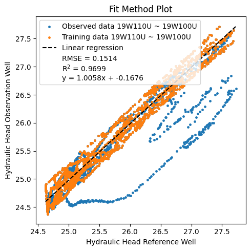
We can see that for the training data, which is data used to fit the regression, our fit seems OK. Observed heads outside of this period show a different behavior - one might suspect a deviation!
Analysing deviations#
Evaluating deviation is a key gwrefpy feature! Below, we plot the resulting fit and transformed head, along with the lower and upper confidence limit based on our p value (0.05) and the fit.
Below, we retrieve the fit from the model and get the associated fitted timeseries for the reference well and the upper and lower bound associated with the p value.
Tip
Below, we generate the plot by hand to showcase how to retrieve the fitted timeseries and its associated upper and lower bound. If you want to quickly review a fit and deviations, use model.plot_fits().
fit = model.get_fits("19W100U")  # we know we only have one fit, so this will be a single object
fitted_ref = fit.get_fit_timeseries()
upper_bound = fit.get_upper_confidence_bound()
lower_bound = fit.get_lower_confidence_bound()

fig, ax = plt.subplots()

_ = ax.fill_between(fitted_ref.index, y1=lower_bound, y2=upper_bound, alpha=0.5)
_ = ax.axvline(pd.Timestamp("2022"), color="black", linewidth=2, label="Calibration stop")


_ = fitted_ref.plot(ax=ax, label="19W100U (fitted)")
_ = obs = model.get_wells("19W110U")
_ = obs.timeseries.plot(ax=ax, label="19W110U")
_ = ax.legend(loc="upper left")
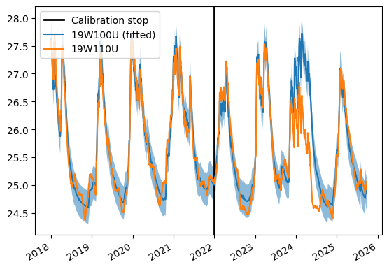
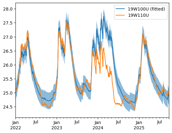
Seems like the observation well (19W110U) dips below the lower bound during 2023 and 2024. Let’s zoom into this period and plot the timesteps where this occurs with a different color after retrivieing them with the get_outliers() method.
fig, ax = plt.subplots()

ax.fill_between(fitted_ref.index, y1=lower_bound, y2=upper_bound, alpha=0.5)

fitted_ref.loc["2022":].plot(ax=ax, label="19W100U (fitted)")
obs.timeseries.loc["2022":].plot(ax=ax, label="19W110U")
_ = ax.legend()
Generate multiple fits at once#
With gwrefpy, you can fit as many reference wells as you like to a single observation well. This is useful if you have many wells to choose from, and would like to rank their fit performance.
Below, we load an example model with many observation and reference wells and clear its existing fits.
large_model = gr.Model("large_example.gwref")
large_model.fits = []
large_model.obs_wells[:3]
[Well(name=01OBS), Well(name=02OBS), Well(name=03OBS)]
We choose a observation well and then run best_fit(), which will default to perform a fit for all available reference wells.
This project many reference wells, so we select only the top 3 fits with remove_fits_by_n() and then plot the resulting regression fit by fit.
_ = large_model.best_fit(obs_well="01OBS", offset="0D")
_ = large_model.remove_fits_by_n("01OBS", 3)

fig, axs = plt.subplots(ncols=len(large_model.fits), sharey=True, figsize=(10,4))
for ax, fit in zip(axs, large_model.fits):
    _ = large_model.plot_fitmethod(fit, ax=ax)
    legend = ax.get_legend()
    legend.set_bbox_to_anchor((0.5, -0.5))
    legend.set_loc("upper center")
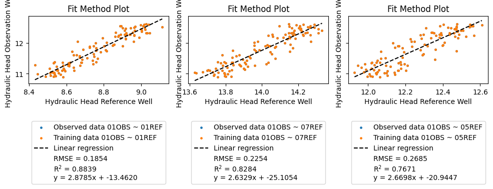
This is a great way to evaluate many reference wells for a single observation well!
Happy fitting!