Quickstart

This quick introductory example demonstrates how to use gwrefpy to analyze an observation and a reference well, calibrate the two wells, and visualize the results.

import gwrefpy as gr
import pandas as pd
import numpy as np

For this quickstart example, we will generate two fictious timeseries.

dates = pd.date_range(start="2020-01-01", periods=365, freq="D")

obs_series = pd.Series(np.sin(np.linspace(0, 4 * np.pi, 365)) + (np.random.normal(0, 0.1, 365) * 2), index=dates)
ref_series = pd.Series(np.sin(np.linspace(0, 4 * np.pi, 365)) + np.random.normal(0, 0.1, 365), index=dates)

To use the timeseries in gwrefpy, we create Well objects.

obs = gr.Well(name="obs", is_reference=False, timeseries=obs_series)
ref = gr.Well(name="ref", is_reference=True, timeseries=ref_series)

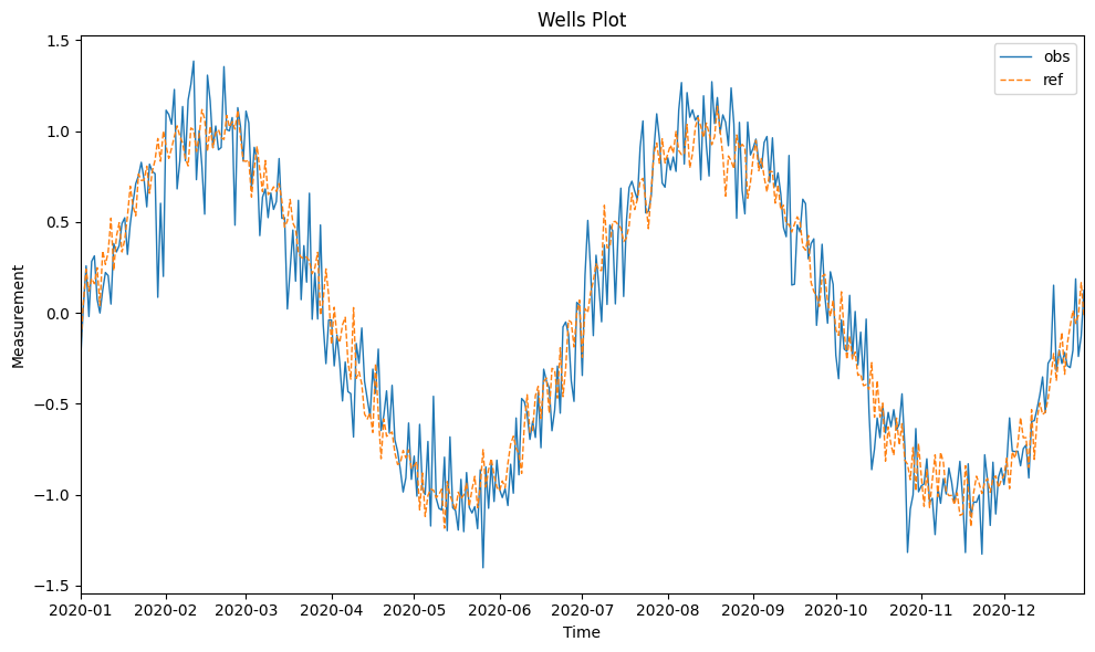
Let’s create our Model object which will hold wells and associated fits. We then add both wells and use model.plot_wells() which will plot all available wells.

model = gr.Model(name="my first model")
model.add_well(obs)
model.add_well(ref)

fig, ax = model.plot_wells()
ax.legend()

Plotting well: obs

Plotting well: ref

<matplotlib.legend.Legend at 0x7f5e20a0e5d0>

Let’s fit the obervation well to our reference well. Since we know the series share the same timestamps, we can safely use "0D" as an offset (i.e., no offset).

See the Regarding time offsets notebook for more details on offsets.

model.fit(
    obs,
    ref,
    offset="0D"
)

tmin is None, setting to min common time of both wells

tmax is None, setting to max common time of both wells

Fitting model 'my first model' using reference well 'ref' and observation well 'obs'.

Fit Results: obs ~ ref

Statistic	Value	Description
RMSE	0.2212	Root Mean Square Error
R²	0.9110	Coefficient of Determination
R-value	0.9544	Correlation Coefficient
Slope	0.9895	Linear Regression Slope
Intercept	-0.0095	Linear Regression Intercept
P-value	0.0000	Statistical Significance
N	365	Number of Data Points
Std Error	0.2218	Standard Error
Confidence	95.0%	Confidence Level

Calibration Period: 2020-01-01 00:00:00 to 2020-12-30 00:00:00
Time Offset: 0D
Aggregation Method: mean

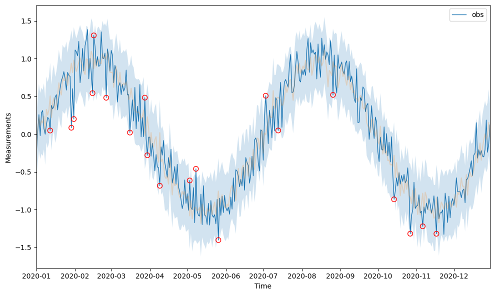
Let’s plot the fit. We can use model.plot_fits() since we only have one fit. By default, any levels from the observation well falling outside the fitted confidence interval will be highlighted with a red circle.

fig, ax = model.plot_fits()
ax.legend()

Plotting fit: obs ~ ref

<matplotlib.legend.Legend at 0x7f5e0719f150>