Working with live data

In this tutorial we will explore how to work with live data when using the gwrefpy package.

This notebook can be downloaded from the source code here.

We will cover the following topics:

1. Create some synthetic live data

2. Create a model and add wells and fit them

3. Update the wells with new data

4. Track the fit quality over time

1. Create some synthetic live data

We start by creating some synthetic data. In a real-world scenario, this data would be read from a database or a file. We will create two sets of data: an initial set and a live set. The initial set will be used to fit the model, and the live set will be used to update the model.

import gwrefpy as gr
import pandas as pd
import numpy as np
gr.set_log_level("ERROR")

ndays_init = 180 # initial data length
ndays_live = 365 # live data length
dates_init = pd.date_range(start="2020-01-01", periods=ndays_init, freq="D") # initial dates
dates_live = pd.date_range(start=dates_init[-1], periods=ndays_live, freq="D") # live dates

# create synthetic data
obs_init = pd.Series(5 + np.sin(np.linspace(0, 4 * np.pi, ndays_init)) + (np.random.normal(0, 0.1, ndays_init) * 2), index=dates_init)
ref_init = pd.Series(10 + np.sin(np.linspace(0, 4 * np.pi, ndays_init)) + np.random.normal(0, 0.1, ndays_init), index=dates_init)
obs_live = pd.Series(5 + np.sin(np.linspace(0, 6 * np.pi, ndays_live)) + (np.random.normal(0, 0.11, ndays_live) * 2), index=dates_live)
# add a drawdown event in the middle of the live data
start = int(ndays_live / 4)
end = int(ndays_live / 2)
half = (end - start) // 2
x = np.concatenate([
    np.linspace(0, 1, half, endpoint=False),
    np.linspace(1, 0, (end - start) - half)
])
obs_live[start:end] -= 1.2 * x**2
ref_live = pd.Series(10 + np.sin(np.linspace(0, 6 * np.pi, ndays_live)) + np.random.normal(0, 0.1, ndays_live), index=dates_live)

2. Create a model and add wells

We add the initial data to the wells and create a model.

well_obs = gr.Well(name="Obs well", is_reference=False, timeseries=obs_init)
well_ref = gr.Well(name="Ref well", is_reference=True, timeseries=ref_init)
model = gr.Model(name="Live data model")
model.add_well([well_obs, well_ref])

We can now fit the model to the initial data.

model.fit(well_obs, well_ref, offset="0D")

Fit Results: Obs well ~ Ref well

Statistic	Value	Description
RMSE	0.2339	Root Mean Square Error
R²	0.8963	Coefficient of Determination
R-value	0.9467	Correlation Coefficient
Slope	0.9574	Linear Regression Slope
Intercept	-4.5678	Linear Regression Intercept
P-value	0.0000	Statistical Significance
N	180	Number of Data Points
Std Error	0.2352	Standard Error
Confidence	95.0%	Confidence Level

Calibration Period: 2020-01-01 00:00:00 to 2020-06-28 00:00:00
Time Offset: 0D
Aggregation Method: mean

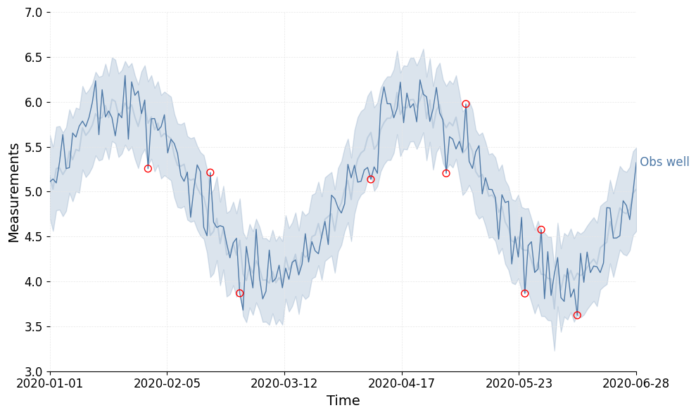
We now take a look at the fit.

_ = model.plot_fits(plot_style="fancy", color_style="color")

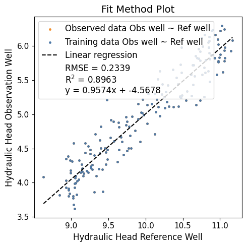
Tip

You can use the plot_fitmethod method to visualize the fit method.

_ = model.plot_fitmethod(plot_style="fancy", color_style="color")

3. Update the wells with new data

We can now update the wells with the live data. This is done by appending the new data to the existing timeseries.

Warning

If the dates in the new data overlap with the existing data an error will be raised. You can supress this error and remove the duplicates by using remove_duiplicates=True argument in the append_timeseries method.

well_obs.append_timeseries(obs_live, remove_duplicates=True)
well_ref.append_timeseries(ref_live, remove_duplicates=True)

We can now plot the updated data.

Tip

You can use the show_initiation_period argument to highlight the initial data period.

_ = model.plot_fits(plot_style="fancy", color_style="color", show_initiation_period=True)
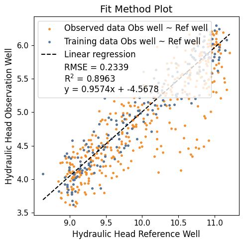
_ = model.plot_fitmethod(plot_style="fancy", color_style="color")

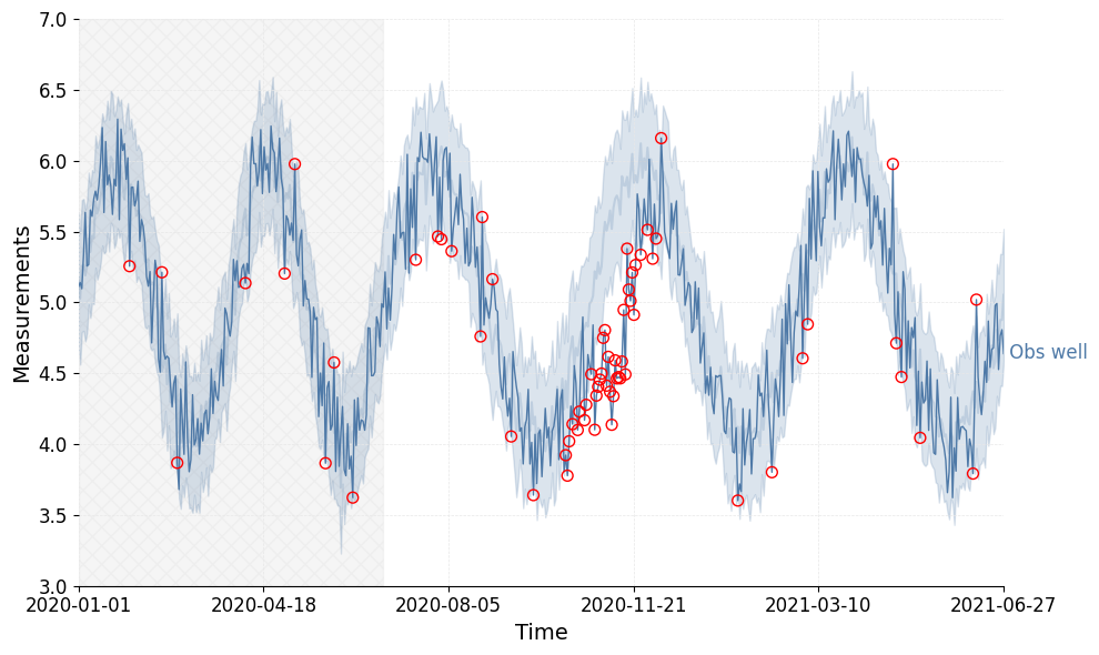
We can see that in the new data we have a drawdown event that is clearly exceeding the prediction interval.

This concludes this notebook on working with live data. Happy coding!